Power Spectral Densities for Continuous Variables

This analysis captures the frequency content of continuous variables.

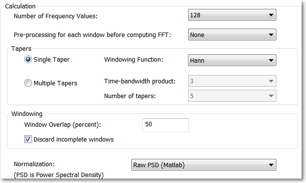
Parameters

Parameter	Description
Number of Fr. Values	Number of values in the spectrum.
Window Overlap (%)	Window (segment) overlap in percent (from 0 to 90).
Window Preprocessing	Preprocessing to be done for each window before calculating the spectrum of the window.
Windowing Function	Windowing Function to be applied to each window before calculating the spectrum of the window.
Discard Incomplete Windows	Option to discard the last window if it contains less than the expected number of data points (less than `NumberOfFrValues*2` points).
Concatenate Selected Data Points	If this option is selected, data points that are selected for analysis (that is, points inside time interval filter) are concatenated and then the PSD of the concatenated signal is calculated. This means that the signal from two adjacent time intervals can be in the same data segment used to calculate FFT. If this option is not selected and interval filter is specified, data segments used to calculate FFT (see Algorithm below) are guaranteed to contain data points from one interval of the interval filter. For each time interval, the first data segment in the interval is aligned with the interval start.
Use Multitaper Algorithm	Option to use multi-taper algorithm.
Time-Bandwidth Product	Time-Bandwidth Product when using multi-taper algorithm.
Number of Tapers	Number of Tapers when using multi-taper algorithm.
Show Frequency From	Minimum frequency to be shown in the spectrum graph.
Show Frequency To	Maximum frequency to be shown in the spectrum graph.
Normalization	Spectrum normalization. See Algorithm below.
Frequency Bands	Percent of spectrum values and the sum of spectrum values will be calculated for each of the specified frequency bands. If Log of PSD Normalization is specified, band percents will be calculated BEFORE applying log() transform.
Log Frequency Scale	An option show Log10 frequency scale.
Smooth	Option to smooth the spectrum after the calculation. See Post-Processing Options for details.
Smooth Filter Width	The width of the smooth filter. See Post-Processing Options for details.
Select Data	If Select Data is From Time Range, only the data from the specified (by Select Data From and Select Data To parameters) time range will be used in analysis. See also Data Selection Options .
Select Data From	Start of the time range in seconds.
Select Data To	End of the time range in seconds.
Interval filter	Specifies the interval filter that will be used to preselect data before analysis. See also Data Selection Options.
Add Freq. Values to Results	An option to add an additional vector of frequency values to the matrix of numerical results.
Send to Matlab	An option to send the matrix of numerical results to Matlab. See also Matlab Options .
Matrix Name	Specifies the name of the results matrix in Matlab workspace.
Matlab command	Specifies a Matlab command that is executed after the numerical results are sent to Matlab.
Send to Excel	An option to send numerical results or summary of numerical results to Excel. See also Excel Options .
Sheet Name	The name of the worksheet in Excel where to copy the numerical results.
TopLeft	Specifies the Excel cell where the results are copied. Should be in the form CR where C is Excel column name, R is the row number. For example, A1 is the top-left cell in the worksheet.

Summary of Numerical Results

The following information is available in the Summary of Numerical Results

Column	Description
Variable	Variable name.
YMin	Spectrum minimum.
YMax	Spectrum maximum.
Filter Length	The length of all the intervals of the interval filter (if a filter was used) or the length or the recording session (in seconds).
Number of FFT windows	Number of FFT windows used in analysis.
Frequency of Minimum	The position of the minimum of the displayed spectrum (in Hz). If there are multiple bins in the spectrum where the spectrum value is equal to the spectrum minimum, this value represents the frequency of the first such bin. If you need to calculate spectrum peaks, go to Post-processing tab, press Post-processing Script Options button and select PostAnalysis_Peaks.py
Frequency of Maximum	The position of the maximum of the displayed spectrum (in Hz). If there are multiple bins in the spectrum where the spectrum value is equal to the spectrum maximum, this value represents the frequency of the first such bin. If you need to calculate spectrum peaks, go to Post-processing tab, press Post-processing Script Options button and select PostAnalysis_Peaks.py

Algorithm

For each selected continuous variable, a standard or multi-taper power spectrum is calculated.

In each case, a Welsh periodogram method is used:

The original data array is split up into data segments (or windows) of length 2*Nf (where Nf is the Number of Frequency Values), overlapping by D points. For example, if overlap is 50%, then D is (2*Nf)/2=Nf.

For each segment, the signal is preprocessed according to Window Preprocessing parameter. For example, if Subtract Mean is selected, ProcessedSignal[i] = Signal[i] - meanOfSignalInSegment.

The overlapping segments are then windowed: after the data is split up into overlapping segments, the individual data segments have a window applied to them (that is, ProcessedWindowedSignal[i] = ProcessedSignal[i]*WindowValue[i]; the window is specified by the Windowing Function).

Most window functions afford more influence to the data at the center of the segment than to data at the edges, which represents a loss of information. To mitigate that loss, the individual data segments are commonly overlapped in time (as in the above step).

After doing the above, the periodogram is calculated by computing the discrete Fourier transform, and then computing the squared magnitude of the result. The individual periodograms are then time-averaged, which reduces the variance of the individual power measurements. The end result is an array of power measurements vs. frequency “bin”.

For multi-taper spectral estimate, several periodograms (tapers) are calculated for each segment. Each taper is calculated by applying a specially designed windowing function (Slepian function, see https://en.wikipedia.org/wiki/Multitaper). All the tapers for a given segment are then averaged to form the periodogram of the segment. The individual segment periodograms are then time-averaged.

See http://www.spectraworks.com/Help/mtmtheory.html for a discussion on selecting Multi-Taper parameters.

Normalization

If Normalization is Raw PSD (Numerical Recipes), the power spectrum is normalized so that the sum of all the spectrum values is equal to the mean squared value of the signal. The formulas (13.4.10) of Numerical Recipes in C are used (squared fft values are divided by N^2 where N is the number of values in data window). (Numerical Recipes in C, Press, Flannery, et al. (Cambridge University Press, 1992)). The units are signal_units^2 (mV^2 in NeuroExplorer). The units in the frequency band sums are mV^2.

If Normalization is % of Total PSD (Numerical Recipes), the power spectrum is normalized so that the sum of all the spectrum values equals 100. The units are %. The units in the frequency band sums are mV^2.

If Normalization is Log of PSD (Numerical Recipes), the power spectrum is calculated using the formula:

power_spectrum[i] = 10.*log10(raw_spectrum[i])

where raw_spectrum is calculated as described above in Raw PSD (Numerical Recipes). The units are dB. The units in the frequency band sums are mV^2.

If Normalization is Raw PSD (Matlab), the power spectrum is normalized as described in https://www.mathworks.com/help/signal/ug/power-spectral-density-estimates-using-fft.html (squared fft values are divided by Fs*N, where Fs is sampling rate, N is the number of values in window, see Matlab code below). The units are signal_units^2/Hz (mV^2/Hz in NeuroExplorer). The units in the frequency band sums are mV^2/Hz.

If Normalization is Log of PSD (Matlab), the power spectrum is calculated using the formula:

power_spectrum[i] = 10.*log10(raw_spectrum_matlab[i])

where raw_spectrum_matlab is calculated as described above in Raw PSD (Matlab). The units are dB/Hz. The units in frequency band sums are mV^2/Hz.

In Matlab:

Fs = 1000;
t = 0:1/Fs:1-1/Fs;
x = cos(2*pi*100*t) + randn(size(t));
xdft = fft(x);
N = length(x);
xdft = xdft(1:N/2+1);

% psdx below corresponds to Raw PSD (Matlab) normalization
% the units are signal_units^2/Hz (mV^2/Hz in NeuroExplorer)
% note that we divide squared fft by (Fs*N)

psdx = (1/(Fs*N)) * abs(xdft).^2;
psdx(2:end-1) = 2*psdx(2:end-1);

% psdDb below corresponds to Log of Raw PSD (Matlab) normalization

psdDb = 10*log10(psdx)

freq = 0:Fs/length(x):Fs/2;

plot(freq,psDb)
title('Periodogram Using FFT')
xlabel('Frequency (Hz)')
ylabel('Power/Frequency (dB/Hz)')

Here is how you can verify that calculations in NeuroExplorer produce the same values as spectrum calculations in Matlab:

Open the file TestDataFile5.nex
Deselect all neuronal variables
Select ContChannel01 variable
Select Matlab | Send Selected Variables to Matlab menu command
Select Power Spectra for Continuous analysis
Specify the following parameters:

Spectral Parameters

Make sure that Add columns(s) with frequency values option is disabled in Post-Processing tab of Analysis Properties dialog
Run the analysis
Select Matlab | Send Numerical Results to Matlab menu command
In Matlab, execute:

p=pwelch(ContChannel01(:,1), hann(256), 128, 256, 10000);

maxDiff = max(abs(p-nex(:,1)))

You will see the following result:

1.3500e-13

This means that at least the first 11 decimal places of the PSD values calculated in NeuroExplorer and in Matlab are identical.