Spectrogram Analysis

This analysis captures the frequency content of continuous variables or neuronal rate histograms.

Parameters

Parameter	Description
Max. Freq.	Maximum frequency for the spectrograms. If at least one continuous variable is selected, the value of the Maximum Frequency parameter is set as 0.5*Digitizing frequency of the first selected continuous variable. All continuous variables selected for this analysis should have the same digitizing rate.
Number of Fr. Values	Number of frequency values.
Normalization	Spectrum units (see Normalization below).
Start	Start of the first window.
Shift Type	Option to specify shift in seconds or as a percent of the sliding window width.
Shift (sec)	If Shift Type is Absolute, specifies how much sliding window is shifted each time (in seconds).
Shift (window %)	If Shift Type is Window Percent, specifies how much sliding window is shifted each time as a percent of the overall sliding window width.
Number of Shifts	total number of sliding windows.
Window Preprocessing	Preprocessing to be done for each window before calculating the spectrum of the window.
Windowing Function	Windowing Function to be applied to each window before calculating the spectrum of the window.
Use Multitaper Algorithm	Option to use multi-taper algorithm.
Time-Bandwidth Product	Time-Bandwidth Product when using multi-taper algorithm.
Number of Tapers	Number of Tapers when using multi-taper algorithm.
Show Freq. From	An option to show a subset of frequencies. Specifies minimum frequency to be displayed.
Show Freq. To	An option to show a subset of frequencies. Specifies maximum frequency to be displayed.
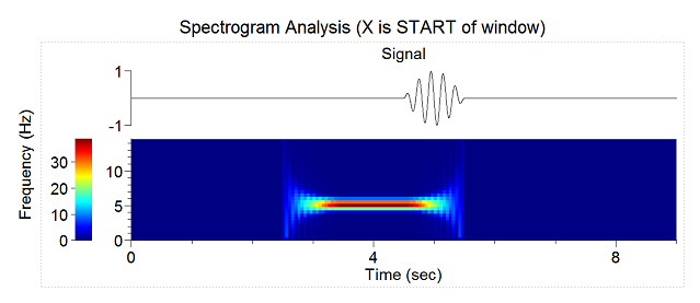
X Axis	Allows to specify what values are shown in the sliding window X axis. There are two options: Start of Window and Center of Window. Suppose your data has the strongest spectral value at 5 seconds. This means that the window that has 5 seconds as its center will show the highest spectrum values. If the window width is 2 seconds, it will be the window [4,6]. If you are using ‘Start of window’ option, you will see the peak at 4 instead of 5 seconds. However, with ‘Center of window’ option, the peak will be at 5 seconds.
Smooth	Option to smooth the spectrum after the calculation. See Post-Processing Options for details.
Smooth Filter Width	The width of the smooth filter. See Post-Processing Options for details.
Color Scale Limit (%)	Specifies maximum value for the color scale in percent. Allows you to ‘zoom in’ small spectrogram values.
Log Vertical Frequency Scale	Option to draw logarithmic vertical frequency scale.
Draw Signal above Spectrogram	Option to draw signal above histogram. The signal is drawn for the time values specified in X Axis. It is recommended to use Center of Window option for X Axis (otherwise, the signal will not be aligned to the spectrogram).
Signal Window Height (%)	The height of the signal window (percent of the total graph window).
Add Freq. Values to Results	An option to add an additional vector (containing a left edge of each frequency bin) to the matrix of numerical results.
Send to Matlab	An option to send the matrix of numerical results to Matlab. See also Matlab Options.
Matrix Name	Specifies the name of the results matrix in Matlab workspace.
Matlab command	Specifies a Matlab command that is executed after the numerical results are sent to Matlab.
Send to Excel	An option to send numerical results or summary of numerical results to Excel. See also Excel Options.
Sheet Name	The name of the worksheet in Excel where to copy the numerical results.
TopLeft	Specifies the Excel cell where the results are copied. Should be in the form CR where C is Excel column name, R is the row number. For example, A1 is the top-left cell in the worksheet.

Summary of Numerical Results

The following information is available in the Summary of Numerical Results

Column	Description
Variable	Variable name.
Y Min	Y axis minimum.
Y Max	Y axis maximum.
Color Scale Min	Color scale minimum.
Color Scale Max	Color scale maximum.
Max Frequency Used	Maximum frequency of the FFTs used.
Rate Histogram Bin	Rate histogram bin size in seconds (if used)
Window width	FFT window width (seconds).
Actual shift	Actual window shift used in analysis.

Algorithm

The power spectrum is calculated for the specified number (Number of Shifts) of windows. For each window:

1. For a timestamped variable, the rate histogram is calculated and copied to the Signal array. The following parameters are used:

Histogram_Start = Start + Shift * (Window_Number - 1)
Bin = 1./(2.*Maximum_Frequency)
NumberOfBins = 2*Number_of_Frequency_Values

2. For a continuous variable,

Window_Start = Start + Shift * (Window_Number - 1)

N values of the continuous variable (starting with the value at Window_Start) are copied to Signal array where N = 2*Number_of_Frequency_Values.

3. Signal values are pre-processed according to the specified Window Preprocessing.

4. Signal values are multiplied by the coefficients of the specified Windowing Function.

5. Discrete FFT of the result is calculated.

6. Power spectrum is calculated from FFT using the formulas defined in (Press et al., Numerical Recipes in C., Cambridge University Press, 1992)

Normalization

If Normalization is Raw PSD (Numerical Recipes), the power spectrum is normalized so that the sum of all the spectrum values is equal to the mean squared value of the rate histogram. The formulas (13.4.10) of Numerical Recipes in C are used. (Numerical Recipes in C, Press, Flannery, et al. (Cambridge University Press, 1992))

If Normalization is % of Total PSD (Numerical Recipes), the power spectrum is normalized so that the sum of all the spectrum values equals 100.

If Normalization is Log of PSD (Numerical Recipes), the power spectrum is calculated using the formula:

power_spectrum[i] = 10.*log10(raw_spectrum[i])

where raw_spectrum is calculated as described above in Raw PSD (Numerical Recipes).

If Normalization is Raw PSD (Matlab), the power spectrum is normalized as described in https://www.mathworks.com/help/signal/ug/power-spectral-density-estimates-using-fft.html

If Normalization is Log of PSD (Matlab), the power spectrum is calculated using the formula:

power_spectrum[i] = 10.*log10(raw_spectrum_matlab[i])

where raw_spectrum_matlab is calculated as described above in Raw PSD (Matlab).